Installing BoofCV on Raspberry PI

Before I talk about getting BoofCV (a computer vision library) up and running, let’s talk about what is needed to get other computer vision libraries running on a Raspberry PI. Then I’ll go over building (not needed), installing (PyBoof technically), and running BoofCV.

Building OpenCV and Other Libraries

For the first time I’m doing actual development on a Raspberry PI and not playing video games. I decided to run a QR Code benchmark I wrote on a desktop computer and see how slow everything is on a Raspberry PI for fun and profit. I have a nifty Python script that builds and runs everything ready to go so this should be a 5 minute task right? Unfortunately this has been bringing back memories of the bad old days when nothing built would build the first time because your setup wasn’t exactly the same as the developers.

First task is to build ZBar. This library hasn’t been maintained in a while and can be tricky to build on a regular desktop. Getting it to compile without errors took an hour or so and who knows how many Google searches. Would have been worse if this was my first time building it and I didn’t have a script that patches the code to fix name conflicts already written.

Second task is installing OpenCV version 3.3.1. That exact version or newer is needed because it contains a fix for jpeg images. As far as I can tell only OpenCV 2.4 is available on apt-get or pip but you might be able to obtain other versions elsewhere, e.g. 3.1.0. Everyone seems to be building it from source. Took me four attempts and about 8 hours to get it working. Build failed a few times (unknown reason or small errors on my part) and built the wrong version of OpenCV once. Now that I know what I’m doing it would take 2 to 3 hours. Most of that is compiling the code.

For sake of being fare, not all libraries are this annoying. SimpleCV can be installed in a few lines using just apt-get according to their instructions.

Building BoofCV

There’s no need to build BoofCV. If you build it from source or download it automatically from Maven Central the code works just the same. It should build out of the box if you’re using Raspbian. If you’re running Ubuntu you need to install Oracle’s JDK because OpenJDK has broken encryption keys and Gradle can’t download the dependencies. If you’re dead set on building BoofCV from source make sure you’re connected to the internet and follow these instructions:

git clone -b master --recursive https://github.com/lessthanoptimal/BoofCV.git boofcv
cd boofcv
./gradlew install

That will download the source code and example data. Example data isn’t required but might be fun to play with. See readme for running examples.

Installing BoofCV

BoofCV is a Java library and you don’t really install it. At least not like a shared library or DLL. It’s either already included in the jar you’re running or you’re building a project and you reference the library using Gradle or Maven. Gradle/Maven will do the hard work for you by automatically downloading all the dependencies. Since this is a non-issue when used as a Java library let’s talk about PyBoof. PyBoof is a Python wrapper around BoofCV and you install that using pip, just like any other Python library.

python3 -m venv venv
source venv/bin/activate
pip install wheel

This should look familiar to almost all python developers. It just sets you up in a safe environment. Wheel is installed because it fixed an issue with the version of pip on my Raspberry PI. Then to install PyBoof just type in the command below. Numpy is a dependency and if you don’t have it installed already this will take a 10 minutes or so to build.

pip install PyBoof==0.29.post3

Now let’s open a image, look for a QR code, and print the results to standard out.

wget https://peterabeles.com/blog/wp-content/uploads/2018/05/qrcode.png

That will download the image for you. Next create a python script with the text below. When you run the script it will pause briefly while it processes the image then print out the results. For best performance process more than one image at a time. The first one is always sluggish.

import numpy as np
import pyboof as pb

# This is needed if you want the code to run fast
pb.init_memmap()

# Load an image as gray scale.=
gray = pb.load_single_band("qrcode.png", np.uint8)

# Declare the QR Code detector
detector = pb.FactoryFiducial(np.uint8).qrcode()

# Process the image, detect the QR Codes, and print the results
detector.detect(gray)
print("Detected a total of {} QR Codes".format(len(detector.detections)))
for qr in detector.detections:
    print("Message: "+qr.message)
    print(" at: "+str(qr.bounds))

Conclusion

BoofCV is very easy to get running on Raspberry PI. Large complex C/C++ projects will take several hours and multiple attempts. Giving you plenty of time to write a blog article.

Gradle: Checking for SNAPSHOT dependencies on a release build

I swear that Gradle used to prevent you from uploading a SNAPSHOT dependency to Maven central in the past. If it ever did, it no longer does as I have screwed up a two times. The reason this is bad is that the SNAPSHOT will eventually expire breaking your project. Thought I was careful on my latest release of BoofCV, but I missed one reference.  Now I have to do a new incremental release, which is a pain and confusing for the users.

To overcome this problem I added the following code to my build.gradle file.  What it does is check all dependencies in each subproject for the word SNAPSHOT.  If one is found it throws an error explaining what happened.

subprojects {
    task checkDependsOnSNAPSHOT << {
        if (version.endsWith("SNAPSHOT"))
            return;

        project.configurations.compile.each {
            if (it.toString().contains("SNAPSHOT"))
                throw new Exception("Release build contains snapshot dependencies: " + it)
        }
    }
    jar.dependsOn checkDependsOnSNAPSHOT
}

This works in Gradle 3.2

Kinect in Java

The folks at OpenKinect did a good job at providing JNI wrappers for their Kinect driver.  What they didn’t do is provide a nice example showing how to process the byte stream data from the RGB and depth cameras.  As far as I can tell, even the comments in their c-code doesn’t fully describe the data format.  The OpenKinect wiki provides a bit more information but tends to be out of date in places and still didn’t fully describe the data format.  So off to google to find a working example in Java.  All I could find was a bunch of stuff telling people to use the Processing OpenKinect code.  That’s of little use to me, but I did find browsing their source code useful.

So for those of you who just want a straight forward example demonstrating how use OpenKinect in Java, you’ve come to the right place.  The code below does use BoofCV for some of the image processing and display, but that’s not essential and could be easily modified to not use BoofCV. 

OpenKinect Version: 0.1.2
BoofCV Version: 0.14

/**
 * Example demonstrating how to process and display data from the Kinect.
 *
 * @author Peter Abeles
 */
public class OpenKinectStreamingTest {

	{
		// Modify this link to be where you store your shared library
		NativeLibrary.addSearchPath("freenect", "/home/pja/libfreenect/build/lib");
	}

	MultiSpectral<ImageUInt8> rgb = new MultiSpectral<ImageUInt8>(ImageUInt8.class,1,1,3);
	ImageUInt16 depth = new ImageUInt16(1,1);

	BufferedImage outRgb;
	ImagePanel guiRgb;

	BufferedImage outDepth;
	ImagePanel guiDepth;

	public void process() {
		Context kinect = Freenect.createContext();

		if( kinect.numDevices() < 0 )
			throw new RuntimeException("No kinect found!");

		Device device = kinect.openDevice(0);

		device.setDepthFormat(DepthFormat.REGISTERED);

		device.setVideoFormat(VideoFormat.RGB);

		device.startDepth(new DepthHandler() {
			@Override
			public void onFrameReceived(FrameMode mode, ByteBuffer frame, int timestamp) {
				processDepth(mode,frame,timestamp);
			}
		});
		device.startVideo(new VideoHandler() {
			@Override
			public void onFrameReceived(FrameMode mode, ByteBuffer frame, int timestamp) {
				processRgb(mode,frame,timestamp);
			}
		});

		long starTime = System.currentTimeMillis();
		while( starTime+100000 > System.currentTimeMillis() ) {}
		System.out.println("100 Seconds elapsed");

		device.stopDepth();
		device.stopVideo();
		device.close();

	}

	protected void processDepth( FrameMode mode, ByteBuffer frame, int timestamp ) {
		System.out.println("Got depth! "+timestamp);

		if( outDepth == null ) {
			depth.reshape(mode.getWidth(),mode.getHeight());
			outDepth = new BufferedImage(depth.width,depth.height,BufferedImage.TYPE_INT_BGR);
			guiDepth = ShowImages.showWindow(outDepth,"Depth Image");
		}

		int indexIn = 0;
		for( int y = 0; y < rgb.height; y++ ) {
			int indexOut = rgb.startIndex + y*rgb.stride;
			for( int x = 0; x < rgb.width; x++ , indexOut++ ) {
				depth.data[indexOut] = (short)((frame.get(indexIn++) & 0xFF) | ((frame.get(indexIn++) & 0xFF) << 8 ));
			}
		}

		VisualizeImageData.grayUnsigned(depth,outDepth,1000);
		guiDepth.repaint();
	}

	protected void processRgb( FrameMode mode, ByteBuffer frame, int timestamp ) {
		if( mode.getVideoFormat() != VideoFormat.RGB ) {
			System.out.println("Bad rgb format!");
		}

		System.out.println("Got rgb! "+timestamp);

		if( outRgb == null ) {
			rgb.reshape(mode.getWidth(),mode.getHeight());
			outRgb = new BufferedImage(rgb.width,rgb.height,BufferedImage.TYPE_INT_BGR);
			guiRgb = ShowImages.showWindow(outRgb,"RGB Image");
		}

		ImageUInt8 band0 = rgb.getBand(0);
		ImageUInt8 band1 = rgb.getBand(1);
		ImageUInt8 band2 = rgb.getBand(2);

		int indexIn = 0;
		for( int y = 0; y < rgb.height; y++ ) {
			int indexOut = rgb.startIndex + y*rgb.stride;
			for( int x = 0; x < rgb.width; x++ , indexOut++ ) {
				band2.data[indexOut] = frame.get(indexIn++);
				band1.data[indexOut] = frame.get(indexIn++);
				band0.data[indexOut] = frame.get(indexIn++);
			}
		}

		ConvertBufferedImage.convertTo_U8(rgb,outRgb);
		guiRgb.repaint();
	}

	public static void main( String args[] ) {
		OpenKinectStreamingTest app = new OpenKinectStreamingTest();

		app.process();
	}
}

BoofCV Android Demo Application

I recently wrote an application to demonstrate some of the capabilities BoofCV on Android.  BoofCV is an open source computer vision library that I’m working on written entirely in Java.  The v0.13 update to BoofCV added functions for converting NV21 images (camera preview format) into BoofCV data types and provided Android specific visualization code.  The end result is that it is now easier to write fast real-time image processing applications on Android using BoofCV.  The source code for the demo application has also be released without restrictions.

General Tips

  • Cell phone cameras are poor quality and suffer from motion blur and rolling shutters.
  • Everything will work better when viewed with good lighting, allowing for faster shutter speeds.
  • When selecting images for association you can swipe to remove previous selection.  Also try tapping and double tapping.
  • Image mosaic and stabilization work best when viewing far away objects, pure rotations, and planar surfaces.
  • When tapping the screen to capture an image, do so gently or else the image will be blurred.
  • On slower devices, pressing the back button to leave a slow process can crash the app and require you to manually kill it.
  • Changing the camera preview size to “large” images can cause out of memory exceptions.

Camera Calibration

Detected square grid pattern.  Red dots show calibration points.

Detected square grid pattern. Red dots show calibration points.

Camera calibration is required for 3D vision applications.  It will allow radial lens distortion to be removed and other intrinsic camera parameters to be known.  To calibrate the camera print out a calibration grid and follow the general instructions from the link below.  Note that the printed image can be rescaled for this application.

http://boofcv.org/index.php?title=Tutorial_Camera_Calibration

After you have printed the calibration target, take pictures of it (by gently tapping the screen) from at least 5 different views and angles.  Most of the pictures should be taken from about 30 degree angle.  When you are done taking pictures, press the “Compute” button to find the intrinsic parameters.  When taking pictures it is recommended that you are sitting down on the ground holding your Android device with both hands.  This is more stable and reduces motion blur, greatly reducing the frustration factor.  Try to fill as much of the screen as possible with the calibration target and if one looks like it might be blurred click the remove button.  On my Sampson Galaxy S3 and Droid 2 I get about 0.2 pixels mean error on good runs and more than a pixel error when things go badly.

Stereo

android_stereo

Stereo depth image computed from two views of the same object. Warmer colors indicate closer objects and color farther away.

Stereo vision allows the scene’s 3D structure to be computed.  This is accomplished using a single camera using taking pictures of the same object two times from two different points of view.  Camera calibration is required before stereo vision can be computed since lens distortion must be removed.  On a Droid 2 cell phone (phone from around 2010/2011) the whole process can take 25 seconds or so, but on a Galaxy S3 (phone from 2012) it only takes four seconds.

To compute a stereo depth image first tap the screen to take a picture. Then move the camera left or right with a little rotation, up/down, and forwards/backwards motion as possible.  How far you should move the camera depends on how far away the objects are.  For close objects 1cm is often good and for objects a few feet away (1 meter) 3cm/1inch works well.  Moving the camera too much tends to be a more common mistake than moving it too little.  It will probably take you a few tries to get a good image.  Also make sure the scene has good texture or else it won’t work.

 Video Mosaic

Mosaic created by moving the camera over a flat table top.

Mosaic created by moving the camera over a flat table top.

Creating a good mosaic can be difficult, with motion blur being the primary culprit.  There is a reason why image stitching software on Android devices use still images.  However with some practice and the right environment you can get some good results.  See the image above.

Remember that it won’t work if you are close up to a complex 3D scene and translating the camera.  Instead try pivoting the camera or working off of far away objects.  Slowly moving the camera also helps.

Rovio to 3D Stereo Point Clouds

rovio_disparity

This disparity image was created using a single Rovio robot by taking pictures from two different locations.

I’m a bit late to the game of Rovio hacking, but here I am experimenting with using a Rovio I bought two years ago.  The Rovio by Wowwee is a remote control car that has a camera mounted on it that can be controlled over wireless web based interface.  When it was discontinued, the existing stock was liquidated in a fire sale, where they were sold for around $100 each.  You can still buy them now, for about $400, on Amazon. Keep in mind you might need to buy a new battery and power supply.

WowWee Rovio Wi-Fi Enabled Robotic WebCam

Picture of a Rovio

Picture of a Rovio

One of the things that makes Rovio so great, and more than a simple toy, is that it can move in any direction! Which means, that unlike your standard remote control car, it can move sideways. This is exactly what you need if you want to do stereo vision and create a point cloud.

The figure to the left shows a disparity image created using a single Rovio by driving it a few inches to the right.  In this disparity image warmer colors are closer and cooler colors are farther away.  See below for the input images.  From this disparity image you can create a point cloud, which can then be used for making 3D models or obstacle detection.  This process is entirely automated using BoofCV and the source code is available online on my Rovio Github project:

https://github.com/lessthanoptimal/rovio
So how does this work?  Well a full explanation would be quite detailed.  The image processing code is for the most part cut and pasted from examples on BoofCV’s website.  A list of relevant example is found below:

 Initial Setup

You will need to do the following once so that your camera is calibrated and that the software knows your robots parameters.

  1. Checkout source code from Github
  2. Calibrate the camera.
    1. Look at this first BoofCV Camera Calibration
    2. Collect images in 640×480 using ManualControlApp by pressing ‘m’
    3. Select good images, run calibration app.  Pixel error should be around 0.3
  3. Get your robots MAC address using ManualControlApp by pressing ‘a’
  4. Create directory for your robot in robots.  Place intrinsic.xml and file “mac” with the MAC address.  See existing examples

Creating Point Cloud

Once you have done all of that all you need to do now is place the Rovio in a well lit room in front of something with lots of texture and run AutoPointCloudApp.  That app will automatically figure out which robot it is controlling, loading calibration, collect and image, move the robot, and collect another image.  The two images are then processed and the results displayed.  Don’t forget to change the IP address in the main() function of AutoPointCloudApp.


rovio_associated

Associated points between the two views using SURF features.

rovio_rectification

Rectified Stereo Images from Rovio


rovio_3d_topview

Synthetic top view created using 3D points computed from the disparity image.


Will Liquidlogic Stand by their Drain Plugs?

Stomper missing its drain plug

Loiquidlogic Stomper missing its drain plug.

At the end of October 2012 my boat finally lost its drain plug. The drain plug had issues almost from the start and never really liked being attached of the boat.  Sometimes it would take a minute or so to screw it in, unless you aligned things just right.  While a minor issue really, things changed when it finally left the boat entirely.  After taking a picture of the boat (right) I felt it was time to contact Liquidlogic and see if they would stand behind their products and provide a new drain plug.  E-mail exchange is posted below.


E-mail exchange with liquidlogic

E-mail exchange with liquidlogic


Conclusion:

While Liquidlogic was very quick to help out and provide a new drain plug, they seemed less inclined to consider related structural damage.  Would have been nice if they replied to the last e-mail. Just in case you are wondering, the drain plug was lost while the boat was stuck underwater for several days.  Swam after my paddle just stuck in a rock on the first rapid in Greatfalls Virginia.

Incorrect Equations in “Review and Analysis of Solutions of the Three Point Perspective Pose Estimation Problem”

In the 1994 paper “Review and Analysis of Solutions of the Three Point Perspective Pose Estimation Problem” by R. M. Haralick, C-N Lee, K. Ottenberg, and M. Nolle, I found a couple of important typos in the equations for the Finsterwalder solution.  This paper describes several solutions to the Perspective Three Point (P3P) problem, two of those solutions I ended up implementing.  The Grunert solution is correct and easy to implement, while the Finsterwalder solution is a little bit more involved.  However since the equations are incorrect for Finsterwalder you could be in for a bit of frustration.

I could not find an e-mail address on the first author’s website.  The paper is also a bit old (but still relevant) and the problem was most likely already reported.  If I’m the first person to notice or try to report the problem after 18 years then it’s a non issue.  However, to help others out there (the one or two which have found this website) here are the corrections:

After it has been corrected, the first line in equation (16) should be:

(b^2 - m^2c^2)u^2 + 2(c^2(cos\beta -n)m - b^2cos\gamma)u

Note that a power of 2 has been added to ‘m’. The equations on the top of the right column of page 337 also needs to be correct and should be:

A = b^2 - m^2c^2
B = c^2(cos\beta -n)m -b^2cos\gamma
C = -c^2 n^2 + 2c^2 n cos\beta + b^2 - c^2

Here a power of two was added to ‘m’ in the first line and ‘c’ in the third line.  Hopefully this post will save someone a few hours of aggravation and deriving equations.


Code from symbolic math using Sage

Abstract

The following article demonstrates how Sage/Python can be used to solve, format, and output auto generated code for complex symbolic equations.   The auto-generated code can be targeted for languages such as C/C++ or Java.  Sage is a computer algebra system (CAS) that uses the Python programming language.  By using Python it is easy to write the code and to take full advantage of Python’s text processing capabilities.

Introduction

It is not uncommon for researchers and engineers to need to solve complex symbolic equations in languages like C/C++ and Java.  While computer algebra systems (CAS), such as Maple or Mathematica, are designed specifically to handle symbolic math with ease, C style languages are not.  A common solution is to first solve the symbolic equations using Maple/Mathematica, then expand out the closed form  solution and convert into compilable code.

This process is often easier said than done.  What was a nice elegant and compact 3 line equation is expanded out into thousands of lines of code.  Hand editing these monstrous equations is not an option.  Another issue is that commercial packages such as Maple and Mathematica are both very expensive.

Recently I needed solve an ugly problem in computer vision and having just learned Python, Sage was the obvious choice.  Sage is CAS which uses Python as its programming language.  Besides being free, Sage is in many ways superior to Maple and Mathematica thanks to Python’s string processing capabilities. The remainder of this article will describe how Sage and Python was used to solve a complex math problem and convert the solution to usable Java code.

The basic for how to use Sage can be found at the following websites:

In this particular application Java code is the final output.  However, it is trivial to convert this example to output C/C++ code.

The Math

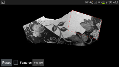
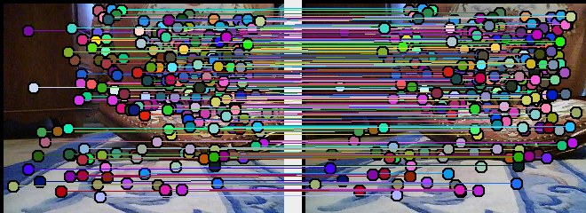
To demonstrate these techniques a complex real-world problem is used.  This problem comes from geometric computer vision and understanding all the math involved is not necessary, but you can find the paper it is based on here [1].  Having an understanding of linear algebra will help you understand all the math terminology.  Briefly stated the problem is to solve for a 3×3 Essential matrix given 5 point correspondences.   If that means nothing to you, don’t worry.

The first step in solving this problem is computing the null space of a 5 by 9 linear system.  The null space is then stored in four column vectors X , Y , Z , and W.  The final solution is a linear combination of these four vectors:

E = x \cdot X + y \cdot Y + z \cdot Z + W

where E is a 3 by 3 Essential matrix being computed, (x,y,z) are the scalar variables being solved for.  Note that the column vectors are converted into a matrix as needed.  Next a system, A, with 10 equations and 20 unknowns is constructed by apply the following constrains on E:

det(E) = 0

E \cdot E^T \cdot E-\frac{1}{2}trace(E \cdot E^T) \cdot E=0

Again if you don’t understand why we are doing the math, don’t panic.  Just know that there are some ugly complex equations which need to be solved for in Java.  In summary we need to do the following:

  • In Java compute the null space and extract out X,Y,Z,W   (Not shown)
  • In Sage construct a system of equation for the above constraints
  • In Sage separate out the known and unknown portions of those equations and output Java code
  • In Java solve for unknowns  (Not shown)

This is actually only 2/3 of the solution.  Since the focus of this article is on the process and not about the details of this particular problem we will skip the rest.

Solving with Sage

All code examples below are written in Python and need to be run inside of Sage’s interactive shell.  Do not try to to run the scripts from Python directly, use Sage.  All python files need the following imports:

from sage.all import *
from numpy.core.fromnumeric import var

The first step in solving this problem is creating several 3×3 symbolic matrices.  Each element in the matrix is unique.  I couldn’t find a function built into Sage, so I wrote my own:

def symMatrix( numRows , numCols , letter ):
 A = matrix(SR,numRows,numCols)
 for i in range(0,numRows):
 for j in range(0,numCols):
 A[i,j] = var('%s%d%d' % (letter,i,j) )
return A

The ‘var’ function is used by Sage to define symbolic variables.  Inside of the Sage interactive shell you can do the following:

sage: A = symMatrix(3,3,'a')
sage: A
[a00 a01 a02]
[a10 a11 a12]
[a20 a21 a22]

Now that you can create a symbolic matrix you can solve rest of the problem as follows:

x,y,z = var('x','y','z')
 
X = symMatrix( 3, 3 , 'X')
Y = symMatrix( 3, 3 , 'Y')
Z = symMatrix( 3, 3 , 'Z')
W = symMatrix( 3, 3 , 'W')
 
E = x*X + y*Y + z*Z + 1*W
EE = E*E.T
 
eq1=det(E)
eq2=EE*E-0.5*EE.trace()*E
 
eqs = (eq1,eq2[0,0],eq2[0,1],eq2[0,2],eq2[1,0],eq2[1,1],eq2[1,2],eq2[2,0],eq2[2,1],eq2[2,2])
 
keysA = ('x^3','y^3','x^2*y','x*y^2','x^2*z','x^2','y^2*z','y^2','x*y*z','x*y')
keysB = ('x*z^2','x*z','x','y*z^2','y*z','y','z^3','z^2','z','')
 
# print out machine code for the linear system
printData('A',eqs,keysA)
printData('B',eqs,keysB)

The functions det and trace compute the determinant and trace of a matrix respectively, A.T is the transpose of A.  Most of that is straight forward algebra, but what about that last bit? Well the printData() function massages those equations to produce usable Java output, which is the subject of the next section.

Generating Code

What the Java code is going to do is solve a linear system. To do that the equations above need to reformatted and converted into matrix format. The variable eqs in the above python code contains equations which have a similar appearance to the equation below on the left, but they need to be expanded out so that they look like the equation on the right.

(1 + 5x)(2 - 3x)(8 + 4y) \rightarrow -60x^2y - 120x^2 + 28xy + 56x + 8y + 16

After the equations have been expanded, the knowns and unknowns are separated and put into matrix format. Consider the system of equations below:

$latex \begin{array}{c}
x + 2xy + 3x^2 = 4 \\
5x + 6xy + 7x^2 = 8 \\
9x + 10xy +11x^2 = 12 \\
\end{array} $

After it has been converted into matrix format it will look like:

$latex A=\left[
\begin{array}{ccc}
1 & 2 & 3 \\
5 & 6 & 7 \\
9 & 10 & 11 \\
\end{array}
\right]
\;\;
B=\left[
\begin{array}{c}
4 \\
8 \\
12 \\
\end{array}
\right]$

At this point the unknowns can be solved for using standard linear algebra tools, e.g. Ax=B.

Part of this process is shown below.  First eq1 is expanded out and then the coefficients of x^3 are extracted.

sage: len(str(eq1))         
465
sage: len(str(eq1.expand()))
7065
sage: extractVarEq(eq1.expand(),'x^3')
'X00*X11*X22 - X00*X12*X21 - X01*X10*X22 + X01*X12*X20 + X02*X10*X21 - X02*X11*X20'

The first two statements are just there to show you how long and ugly these equations are.  Below is the python code for extractVarEq:

def extractVarEq( expression , key ):
  chars = set('xyz')
  # expand out and convert into a string
  expression = str(expression.expand())
  # Make sure negative symbols are not stripped and split into multiplicative blocks
  s = expression.replace('- ','-').split(' ')
  # Find blocks multiplied by the key and remove the key from the string
  if len(key) == 0:
    var = [w for w in s if len(w) != 1 and not any( c in chars for c in w )]
  else:
    var = [w[:-(1+len(key))] for w in s if (w.endswith(key) and not any(c in chars for c in w[:-len(key)])) ]
 
  # Expand out power
  var = [expandPower(w) for w in var] 
 
  # construct a string which can be compiled
  ret = var[0]
  for w in var[1:]:
    if w[0] == '-':
      ret += ' - '+w[1:]
    else:
      ret += ' + '+w
 
  return ret

The function expandPower(w) converts statements like a^3 into a*a*a which can be parsed by Java.  After processing all 10 equations most of the hard work is done,   Addition processing is done to simplify the equations, but the code is a bit convoluted and isn’t discussed here.  The final output it sent into a text file and then pasted into a Java application.

Want to see what the final output looks like? Well here is a small sniplet:

A.data[0] = X20*( X01*X12 - X02*X11 ) + X10*( -X01*X22 + X02*X21 ) + X00*( X11*X22 - X12*X21 );
A.data[1] = Y02*( Y10*Y21 - Y11*Y20 ) + Y00*( Y11*Y22 - Y12*Y21 ) + Y01*( -Y10*Y22 + Y12*Y20 );
A.data[2] = X22*( X00*Y11 - X01*Y10 - X10*Y01 + X11*Y00 ) + X20*( X01*Y12 - X02*Y11 - X11*Y02 + X12*Y01 ) + X21*( -X00*Y12 + X02*Y10 + X10*Y02 - X12*Y00 ) + X01*( -X10*Y22 + X12*Y20 ) + Y21*( -X00*X12 + X02*X10 ) + X11*( X00*Y22 - X02*Y20 );

The full source code can be downloaded from:

[1] David Nister “An Efficient Solution to the Five-Point Relative Pose Problem” Pattern Analysis and Machine Intelligence, 2004

Inverse Radial Distortion Formula

Where are the inverse equations hiding?

A common problem in computer vision is modelling lens distortion.  Lens distortion distort the shape of objects and introduce large errors in structure from motion applications.  Techniques and tools for calibrating cameras and removing lens distortion are widely available.  While books and papers readily provide the forward distortion equations (given an ideal undistorted coordinate, compute the distorted coordinate) inverse equations are much harder to come by.

Turns out there is no analytic equation for inverse radial distortion.  Which might explain the mysterious absence of inverse equations, but still it would be nice if this issue was discussed in common references. First a brief summary of background equations is given, followed by the solution to the inverse distortion problem.

Inverse Distortion Problem: Given a distorted image coordinate and distortion parameters, determined the coordinate of the ideal undistorted coordinate.

Background

Unlike the idealized pin-hole camera model, real world cameras have lens distortions.  Radial distortion is a common model for lens distortion and is summarized by the following equations:

\hat{x} = x + x[k_1 r^2 + k_2 r^4]
\hat{u} = u + (u-u_0)[k_1 r^2 + k_2 r^4]
r^2=u_x^2 + u_y^2

where \hat{u}=[\hat{u}_x,\hat{u}_y] and u are the observed distorted and ideal undistorted pixel coordinates, \hat{x} and x are the observed and ideal undistorted normalized pixel coordinates, and k_1, k_2 are radial distortion coefficients.  The relationship between normalized pixel and unnormalized pixel coordinates is determined by the camera calibration matrix, u=C x, where C is the 3×3 calibration matrix.

Solution

While there is no analytic solution there is an iterative solution.  The iterative solution works by first estimating the radial distortion’s magnitude at the distorted point and then refining the estimate until it converges.

  1. x=C^{-1}\hat{u}
  2. do until converge:
    1. r=||x||^2
    2. m=k_1 r^2 + k_2 r^4
    3. x=\frac{C^{-1}\hat{u}}{1+m}
  3. u = \frac{x+x_0 m}{1+m}

Where x_0 is the principle point/image center, and ||x|| is the Euclidean norm. Only a few iterations are required before convergence.  For added speed when applying to an entire image the results can be cached.  A similar solution can be found by adding in terms for tangential distortion.


Converting X-Ray Images into JPEG

While out scouting a rapid on the North Fork of the Stanislaus in California I decided to take a closer look at the rocks down below by flinging my body rapidly face first into them.  Some people might have mistaken this action for slipping.  While doing so I twisted my middle finger and it has been swollen ever since.  Hasn’t bother me much but my doctor thought I should get it x-rayed to be safe.

One-finger salute X-Ray. There was no fracture.

This is how I came across a CD full of hand x-rays.  Now most people would use a standardized format that everyone can understand.  Being the medical field they have their own format to encapsulate standard formats and make them unreadable.  All of these files had a ‘dcm’ extension, which means they contain DICOM image files.  A quick search online turned up several suggestions on how to convert the file and none of them worked.

Using the unix “convert” command might have worked, but there seems to be problems if a loss less JPEG is encapsulated in the DICOM file.  A bit more searching and I found out about dcmtk which is an open source project for reading and modifying these files.  It provides several functions, such “dcm2pdf” or “dcmdjpeg” but these won’t create a jpeg directly.  The command ‘dcmdump’ shows information on the file and verified that it was in fact in lossless jpeg format.  To extract a readable image from the DICOM file, follow these steps in Linux:

  1. install dcptk
  2. dcmdump INPUT.dcm
  3. dcmdjpeg INPUT.dcm OUTPUT.dcm
  4. dcmp2pgm OUTPUT.dcm image.pgm

The second step verifies which image format is encapsulated and is used to determine which dcmd* command should be invoked.  The third step converts the jpeg encoded DICOM into a standard format DICOM file.  The fourth step converts the DICOM file into a ‘pgm’ file.  The pgm file can be viewed in most graphics program and can be easily converted into a jpeg file.  To the right is one of the extracted x-ray images.